Denoising Diffusion Probabilistic Models (DDPM) 논문 리뷰

최근, generative model에서 가장 많이 사용되고 있는 diffusion model을 다루게 되면서 가장 기초적인 diffusion model부터 공부를 하기 시작했다. 새로 들어간 랩실에서 감사하게도 diffusion 스터디가 열려서 수식 유도와 함께 논문 내용들을 살펴보고자 한다.

 

[논문링크]

https://arxiv.org/pdf/2006.11239.pdf

 

공부하다가 모르는 단어들에 대한 정리

 

논문을 읽던 도중에 이해가 되지 않는 단어들이 많았다. 특히, 이쪽 분야의 논문을 읽으면서 느낀 점들은 우리가 실제로 사용하는 영어 단어와 의미가 조금 다르게 사용되는 용어들이 많다는 것이다. 그래서 단어에 대한 내용들을 미리 짚고 넘어가면 좋을 것 같아서, 논문을 읽다가 몰랐던 단어들에 대해 나름대로의 정리를 해보았다. 오류가 있을 수도 있으니 피드백 해주시면 감사하겠습니다.

• weighted variational bound
  • 정확하게 이런 용어가 존재한다기 보다, 가중치를 부여한 variational inference에서 사용되는 bound들을 결정하는 것 같음
  • variational method란, 함수를 변수처럼 취급하여 문제를 해결하는 방식을 의미한다.
    • 이미 알고 있는 식에 대해서 KL-divergence를 활용하여 approximation을 시도
    • 해당 방법론에 사용되는 식들은 ‘물리학’에서 사용되는 개념들이며, entropy의 개념을 확장해서 사용 → variational free energy라고 부르기도 함 (그래서 energy-based model이라고 하는걸까?)
• energy-based model
  • learning을 energy 관점에서 보면 데이터를 바탕으로 어떤 energy surface를 만들고 여기서 데이터에 가까울수록 energy를 낮게, 멀수록 energy를 높게 할당하여 인코딩하는 모델을 의미한다.
    • energy function : data에 대해 energy 값을 반환하는 함수
    • 데이터에 가까울수록 energy를 낮게 설정하는 것은 energy가 낮을수록 안정적인 ‘물리학’에서의 개념을 차용한 것으로 보임.
• denoising score matching
  • data로부터 noise를 제거하는 방법으로 학습하는 기법을 의미한다. 원본 데이터의 PDF를 모델링하지 않고 데이터의 score를 모델링한다.
    • 여기서 score는 gradient, log likelihood function의 미분 값 등이 될 수 있다.
• latent variable models (↔ autoregressive model)
  • 직접 관찰되지 않는 변수들, 즉 latent variable을 가정하여 사용하는 모델을 의미한다. 모든 random variable이 관찰될 수 있는 autoregressive model은 tractable한 density를 가지지만, latent variable model은 random variable의 일부는 보이지 않기 때문에 hidden 상태로 두고 intractable density를 가정한다.
  • 왜 latent variable model을 사용할까?
    • data를 low-dimension에서 representation할 필요가 종종 있기 때문이다.
    • autoregressive는 sampling이 느린 반면, latent variable model은 통계적인 패턴을 활용한 빠른 sampling을 할 수 있다.
    • 일부 latent variable을 conditional하게 넣어 활용할 수 있다. → 이 부분은 이해가 잘 안됨.
• Rao-blackwellized fashion
  • Gaussian distribution이므로 VAE처럼 reparameterization trick으로 KL-divergence term을 학습 → closed form을 활용하는데 이 때, 이 term들은 monte carlo estimates 대신 사용이 가능하다.
• Langevin dynamics
  • 일반적으로 물리학에서 쓰이는 역학이며, 브라운 운동을 stochastic process로 나타내는 미분 방정식을 의미한다.
• lossy compression
  • signal compression에서 사용되는 용어이며, 데이터의 일부 정보를 손실하면서 데이터를 압축하여 압축률을 높이는 방법을 의미한다. 이로 인해 데이터를 완전히 복구할 수 없다.
• lossless codelength
  • lossless compression은 원본 데이터를 완전히 복구할 수 있는 압축 방법이며 이 때, code length를 lossless codelength라고 한다.

 

이제 본격적으로 논문 내용들을 살펴보자.

 

Abstract

• diffusion probabilistic model (DPM) 을 사용하여 높은 퀄리티의 이미지 합성을 하는 방법을 제시
  • 일종의 latent variable model이며 nonequilibrium thermodynamics로부터 영감을 받음
• DPM과 denoising score matching 사이의 novel connection에 따라 디자인된 weighted variational bound로 훈련
• autoregressive decoding의 일반화로 해석할 수 있는 lossy decompression scheme을 admit

Introduction

 

• 모든 종류의 Deep generative model은 높은 수준의 sample들을 생성
  • GANs / autoregressive models / flows / variational autoencoder (VAEs)
• 또한, energy-based modeling과 score matching에서 눈에 띄는 발전을 이룸
  • 이 부분들에 대해서는 추후에 다루게 될 score-based diffusion model에서 자세하게 언급된다.

• 이 paper에서는 diffusion probabilistic model (diffusion model)을 제시함
• diffusion model이란, variational inference를 사용하여 훈련된 parameterized Markov chain
  • finite time동안 data와 matching되는 sample 생성
• transition of chain은 diffusion process를 reverse하는 방법을 학습한다
  • diffusion process : signal이 destroyed 될 때까지 sampling의 반대 방향으로 data에 noise를 점차 추가하는 방식
  • 여기서 transition은 한 state에서 다음 state로 넘어가는 것을 의미
• diffusion이 적은 양의 gaussian noise로 구성될 때, sampling chain transition을 conditional gaussian으로 설정해도 충분 → 간단한 neural network를 parameterization하는 것이 가능
• diffusion model은 정의하기 쉽고 훈련하기에도 효율적이지만, 높은 수준의 sample들을 생성할 수 있다는 것에 대한 demonstration 없다.
  • 아마 정확한 증명 과정이 없다는 것을 의미하는 것 같다.
• diffusion model이 실제로 높은 수준의 sample을 만들 수 있으며 때때로 다른 모델보다 더 좋은 결과를 얻을 수 있다.
• 게다가 diffusion model의 특정 parameterization이 training동안의 여러 noise level을 denoising score matching 하는 것 + sampling동안 annealed langevin dynamics하는 것과 같음을 확인
  • 이 parameterization을 사용하여 최고의 결과를 낼 수 있었으며 이는 이 paper의 주요 contribution중 하나이다.
• 하지만 diffusion model은 다른 likelihood-based model에 비해 competitive log likelihood를 가지고 있지 않다.
• diffusion model의 lossless codelengths의 대부분이 보이지 않는 이미지의 detail을 묘사하는 데에 사용되고 있음을 확인했다.
• 이 현상에 대해 more refined 분석을 제시하며 diffusion model의 sampling 과정이 bit 순서에 따른 autoregressive decoding과 유사한 progressive decoding의 일종임을 보여준다.
  • 여기서 progressive decoding은 일반적으로 autoregressive model에서 가능한 것보다 훨씬 더 광범위하게 generalization이 된 decoding이라는 것을 의미한다.

 

2. Background

 

• Diffusion model은 $p_\theta(\mathbf{x_0}) := \int p_\theta(\mathbf{x_{0:T}})d\mathbf{x_{1:T}}$ 형태의 latent variable models이다
  • 여기서 $\mathbf{x_1},…,\mathbf{x_T}$는 data인 $\mathbf{x_0}\sim q(\mathbf{x_0})$과 같은 dimension인 latent를 의미한다.
  • 즉, 원본 이미지를 만들기 위해 noise image에서 noise를 제거해 나가는 과정
  • joint distribution인 $p_\theta(\mathbf{x_{0:T}})$은 reverse process라고 부르며 이는 $p(\mathbf{x_T}) = \mathcal{N}(\mathbf{x_T};\mathbf{0,I})$에서 시작하는 learned gaussian transition을 가진 markov chain으로 정의할 수 있다.
    • $p(\mathbf{x_T}) = \mathcal{N}(\mathbf{x_T};\mathbf{0,I})$는 $p(\mathbf{x_T})$가 평균이 0이고 covariance matrix가 $\mathbf{I}$인 normal distribution을 따른다는 것을 의미한다.
  • $p_\theta(\mathbf{x_{0:T}}) := p(\mathbf{x_T})\prod^T_{t=1}p_\theta(\mathbf{x_{t-1}}|\mathbf{x_t}), \\ p_\theta(\mathbf{x_{t-1}|x_t}):=\mathcal{N}(\mathbf{x_{t-1};\mu_\theta(x_t,}t),\sum_\theta(\mathbf{x_t},t))$
    • 첫번째 식은 $x_T$부터 markov chain을 통해 $x_0$까지를 얻는 과정
    • 두번째 식은 각 conditional probability가 시간 t에서 state $\mathbf{x_t}$가 주어졌을 때, $\mu$와 $\sum$을 가지는 정규 분포를 따른다는 것을 의미한다.
• diffusion model이 다른 latent variable model과 구분되는 점은 forward process or diffusion process 라고 불리는 대략적인 posterior $q(\mathbf{x_{1:T}|x_0})$가 variance schedule $(\beta_1,…\beta_T)$에 따라 데이터에 점차 gaussian noise를 더해가는 markov chain에 고정되어 있다는 점이다. ⇒ 여러 time-step으로 noise를 단계별로 추가하는 것을 하나의 step으로 처리한다는 점이 DDPM의 주된 원리
  • $q(\mathbf{x_{1:T}|x_0}) := \prod^T_{t=1}q(\mathbf{x_t|x_{t-1}}),\\ q(\mathbf{x_t|x_{t-1}}):=\mathcal{N}(\mathbf{x_t;\sqrt{1-\beta_t}x_{t-1},\beta_t,I})$
    • 첫번째 식은 posterior가 markov chain의 형태로 이루어져 있음을 의미한다.
    • 두번째 식은 각각의 conditional probability에서 $\mathbf{x_{t-1}}$이 주어졌을 때 $\mathbf{x_t}$는 $(\sqrt{1-\beta_t}\mathbf{x_{t-1}},\beta_t\mathbf{I})$를 가지는 정규 분포를 따른다는 것을 의미한다.
    • 즉, 1에 가깝도록 이전 이미지의 정보를 반영하고 아주 작은 $\beta_t$값만큼 noise를 추가하는 식이다.
  • variance schedule $(\beta_1,…,\beta_T)$는 각 단계에서 추가되는 노이즈의 양을 의미한다. 모델이 데이터에 노이즈를 추가하는 과정에서 노이즈의 분산을 시간에 따라 조정하는 것을 의미한다. → hyperparameter 값이다.
• training은 negative log likelihood에 대한 일반적인 variational bound를 optimizing하는 것으로 진행된다.
  • $\mathbb{E[-log\space p_\theta(\mathbf{x_0})]\leq E_q[-log \frac{p_\theta(\mathbf{x_{0:T})}}{q(\mathbf{x_{1:T}|x_0})}] = E_q[-log\space p(\mathbf{x_T})-\sum_{t \geq 1}log\frac{p_\theta(\mathbf{x_{t-1}|x_t})}{q(\mathbf{x_t|x_{t-1}})}]} =: L$ → extra information에 Extended derivation (p.13)에 추가 설명 있음.
• forward process variance $\beta_t$는 reparameterization에 의해 학습이 가능하다, 혹은 hyperparameter로써 상수 값으로 두어도 좋다.
• 그리고 reverse process의 expressiveness는 $p_\theta(\mathbf{x_{t-1}|x_t})$에서 gaussian conditional 선택에 의해 보장된다.
  • 그 이유는 forward / reverse process 모두 $\beta_t$가 작을 때, 같은 functional form을 가지기 때문이다.
  • 여기서 $p_\theta(\mathbf{x_{t-1}|x_t})$가 gaussian 형태로 modeling이 되는 것이 gaussian conditional이다.
• forward process의 주목할만한 성질은 forward process가 임의의 timestep t에서 $x_t$를 closed form으로 sampling할 수 있다는 것이다.
  • $q(\mathbf{x_t|x_0}) = \mathcal{N}(\mathbf{x_t;\sqrt{\bar{\alpha_t}}x_0,(1-\bar{\alpha_t})I)}$
• 따라서 효율적인 training이 가능하다 ← stochastic gradient descent로 L의 random term을 optimizing할 수 있기 때문
• 또한, L을 rewriting함으로써 variance reduction으로부터 추가적인 improvement를 얻을 수 있다.
  • $\mathbb{E_q}[D_{KL}(q(\mathbf{x_T | x_0) || p(x_T)}){(=L_T)} + \sum{t>1} D_{KL}(q(\mathbf{x_{t-1} | x_t, x_0) || p_\theta(x_{t-1} | x_t)}){(=L{t-1})} - \log p_\theta(\mathbf{x_0 | x_1})_{(=L_0)}]$
  • 이 식은 forward process posterior와 $p_\theta(\mathbf{x_{t-1}|x_t})$를 직접 비교하기 위해 KL divergence를 사용했으며 이는 $x_0$에서 conditioned 되었을 때 tractable할 수 있다.
    • which is tractable when conditioned on $\mathbf{x_0}$ → $\mathbf{x_0}$에 다음과 같은 조건을 주었을 때, tractable하다.
    • $q(\mathbf{x_{t-1}|x_t,x_0}):=\mathcal{N}(\mathbf{x_{t-1};\tilde{\mu_t}(x_t,x_0),\tilde{\beta_t}I})$
      • $\mathbf{\tilde{\mu_t}(x_t,x_0)}:= \frac{\sqrt{\bar{\alpha}_{t-1}}\beta_t}{1-\bar{\alpha}t}\mathbf{x_0} + \frac{\sqrt{\alpha_t}(1-\bar{\alpha}{t-1})}{1-\bar{\alpha}t}\mathbf{x_t}, \\ \tilde{\beta_t}:=\frac{1-\bar{\alpha}{t-1}}{1-\bar{\alpha_t}}\beta_t$
• 결론적으로 모든 KL divergences는 gaussian들 사이의 comparison이다, 따라서 이 식들은 high variance Monte Carlo estimates 대신에 closed form expression과 함께 Rao-Blackwellized fashion에서 계산할 수 있다.

 

3. Diffusion models and denoising autoencoders

Diffusion model은 latent variable models의 restricted class처럼 보이지만 implementation에 있어서 굉장히 큰 자유도를 보여준다.

forward process, model architecture, reverse process의 gaussian distribution parameterization에 사용되는 variance, $\beta_t$를 반드시 설정해야 한다. paper에서의 choice를 따라오기 위해서, diffusion model과 denoising score matching 사이의 explicit connection을 제시한다.

3.1 Forward process and $L_T$

forward process variance \beta_t를 reparameterization으로 학습 가능하며 constant로 고정을 해둔 덕분에 approximate posterior, q는 learnable parameter를 가지지 않으며 따라서 $L_T$는 훈련 과정 중에서 constant이므로 무시할 수 있게 된다.

3.2 Reverse process and $L_{1:T-1}$

이제 우리는 $p_\theta(\mathbf{x_{t-1}|x_t})= \mathcal{N}(\mathbf{x_{t-1};\mu_\theta(x_t},t),\sum_\theta(\mathbf{x_t},t))$ $(1<t\leq T)$ 를 어떻게 선택할 것인지부터 논의해야 한다.

• 가장 처음에는 $\sum_\theta(\mathbf{x_t},t) = \sigma^2_t\mathbf{I}$로 설정한다.
  • 실험해보았을 때, $\sigma^2_t = \beta_t \space or \space \tilde{\beta}_t$는 비슷한 결과를 보인다.
  • 따라서 첫번째 선택은 $\mathbf{x_0}\sim\mathcal{N}(\mathbf{0,I})$로 최적화 된다.
  • 2번째 선택은 한 점으로 deterministically하게 최적화 된다.
    • 이 2가지 extreme choice는 각각 데이터에 대한 reverse process entropy의 upper bound와 lower bound와 일치한다.
• 두번째로, $\mu_\theta(\mathbf{x_t},t)$를 표현하기 위해서 특정한 parameterization을 제시한다. 이는 $L_t$의 분석에 따라 만들어 졌다.
  • $L_{t-1} = \mathbb{E}_q[\frac{1}{2\sigma^2_t}||\tilde{\mu}t(\mathbf{x_t,x_0}-\mu\theta(\mathbf{x_t},t)||^2]+C$
    • C는 $\theta$에 의존적이지 않은 constant를 의미한다.
  • 따라서 우리는 $\mu_\theta$의 가장 직관적인 parameterization이 $\tilde{\mu}_t$를 예측하는 모델임을 알 수 있다.
  • 이 식을 $q(\mathbf{x_t|x_0}) = \mathcal{N}(\mathbf{x_t;\sqrt{\bar{\alpha_t}}x_0,(1-\bar{\alpha_t})I)}$을 이용해 reparameterizing을 진행하면 다음과 같이 확장할 수 있다.

이 식을 통해 \mu_\theta가 반드시 \frac{1}{\sqrt{\alpha_t}}(\mathbf{x_t}-\frac{\beta_t}{\sqrt{1-\bar{\alpha_t}}}\epsilon_\theta(\mathbf{x_t},t))를 예측해야 함을 알 수 있다. \mathbf{x_t}는 모델의 input으로 사용 가능하므로 우리는 다음과 같은 parameterization을 선택할 수 있다.

• $\epsilon_\theta$는 $\mathbf{x_t}$로부터 $\epsilon$을 예측하기 위한 function approximator를 의미한다.
• 즉, $\mathbf{x_{t-1}}$을 sampling하는 것은 eq(11)의 마지막 항 + $\sigma_t\mathbf{z}$를 계산하는 것과 같다. $(\mathbf{z}\sim \mathcal{N}(\mathbf{0,I}))$

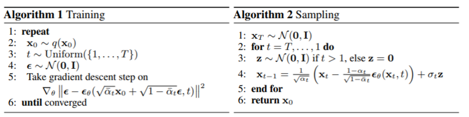
• complete algorithm은 위와 같으며, algorithm 2는 Langevin dynamics와 비슷한 형태를 보인다.
  • data density로부터 학습한 gradient로써 $\epsilon_\theta$를 활용하는 Langevin dynamics
• 여기서 더 나아가, eq (11)을 parameterization하면 eq(10)을 다음과 같이 간소화 할 수 있다.

• 이는 시간에 따라 여러 noise scale을 거친 denoising score matching과 닮은 형태이다.
• (12)가 (11)의 variantional bound와 일치하므로, 우리는 denoising score matching과 유사한 objective를 최적화 하는 것이 결국 variational inference를 사용해서 한정된 time-marginal의 sampling chain (Langevin dynamics와 유사한) 을 fitting하는 것과 같음을 알 수 있다.

요약하자면, $\tilde{\mu_t}$를 예측하기 위해 reverse process mean function approximator, $\mu_\theta$를 학습할 수 있으며 혹은 parameterization을 수정하여 $\epsilon$을 예측하도록 학습 시킬 수도 있다.

• ($\mathbf{x_0}$을 예측할 가능성도 있지만 이는 sample quality를 악화시킨다는 것을 실험 초기에 발견했다.)

$\epsilon$ prediction parameterization이 Langevin dynamics와 유사하고 diffusion model의 denoising score matching과 유사한 variational bound를 단순화한다는 것을 밝혔다. 비록 단순한 parameterization일지 몰라도 이에 대한 효율성은 section 4에서 다룬다.

3.3 Data scaling, reverse process decoder, and $L_0$

image는 0~255까지의 정수로 이루어져 있다. 이를 [-1,1]로 linearly하게 scaling했으며 이는 neural network reverse process가 standard normal prior로부터 항상 일정하게 작동하도록 만들어 준다.

discrete log likelihood를 얻기 위해서 reverse process의 마지막 term에 gaussian $\mathcal{N}(\mathbf{x_0;\mu_\theta(x_1,1),\sigma^2_1I})$으로부터 얻은 independent discrete decoder를 추가해준다.

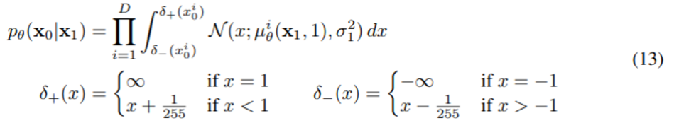
• D : data dimensionality
• i superscript : 좌표축 하나를 extraction한 것
  • conditional autoregressive model과 같이 더 강력한 decoder를 incorporate → future work
• VAE decoder와 autoregressive model에서 사용되는 discretized continuous distribution과 비슷하게, 우리의 선택은 variational bound가 discrete data의 lossless codelength라는 것을 보장한다.
  • 이 때, data에 noise를 추가할 필요성 or log likelihood에 Jacobian scaling operation을 추가하는 것은 X
• sampling 마지막에 우리는 $\mu_\theta(\mathbf{x_1},1)$이 noiselessly 함을 보여준다.

3.4 Simplified training objective

위에서 정의한 reverse process와 decoder와 함께, eq(12), (13)에서 유도한 term들로 구성된 variational bound는 $\theta$에 대해서 미분 가능하며 training을 위해 사용될 수 있다.

하지만 sample quality를 향상시키고 더 구현하기 쉽게 하기 위해서는 variational bound를 다음과 같이 변형하는 것이 더 유익함을 발견했다.

• t는 1~T까지 uniform한 distribution을 갖는다.
  • t=1인 case는 bin width와 gaussian probability density function을 곱한 것으로부터 추정된 discrete decoder definition (13)에서의 integral을 포함한 L_0와 같다.
    • 이때, t=1이라는 것은 특정 시점을 의미하며 $\sigma^2_1$와 edge effects를 무시할 수 있다.
  • t>1인 case는 NCSN denoising score matching model에서 사용된 loss weighting과 유사한 Eq (12)의 unweighted version과 같다.
    • t>1이라는 것은 다른 시점을 의미한다.
    • $L_T$는 $\beta_t$가 고정되어 있으므로 forward process에서 나타나지 않는다.
• 간소화된 objective인 eq(14)가 eq(12)에서 weighting을 생략함으로써, standard variational bound와 비교했을 때 reconstruction의 다른 측면들을 강조하는 weighted variational bound임을 알 수 있다.
  • 특히 우리의 diffusion process setup은 small t와 일치하는 loss term에 가중치를 낮게 주어 simplified objective를 유도한다.
• 이런 term들이 매우 적은 양의 noise가 있는 데이터에서 denoising을 할 수 있게 훈련시키기 때문에 가중치를 적게 부여해서 더 큰 t에 대해 더 어려운 denoising 작업도 수행할 수 있도록 한다.

 

4. Experiments

 

기본적인 세팅은 다음과 같다.

• T : 1000
• $\beta_1 = 10^{-4} \sim \beta_T = 0.02$
• Backbone : U-Net (similar to unmasked PixelCNN++)

4.1 Sample quality

 

Table 1은 CIFAR10 dataset에 대한 여러가지 score를 보여주고 있다.

여기서 FID score는 원본 이미지와 생성된 이미지 간의 유사성 거리를 의미하며, 이 거리가 짧을수록 유사하다고 판단하기 때문에 FID score는 낮을 수록 더 좋다고 평가한다.

4.2 Reverse process parameterization and training objective ablation

Table 2는 reverse process parameterization과 training objective의 sample quality effect에 대한 결과이다.

• baseline은 eq(14)와 유사한 unweighted mean squared error 대신 true variational bound에서 train될 때만 잘 작동
• 또한 learning reverse process variance가 불안정한 training을 유발하고 variance를 fix했을 때보다 quality도 떨어짐.
• 하지만 paper에서 제안한 것처럼 $\epsilon$을 예측하는 것은 고정된 variance에서 variational bound를 학습 시킬 때, $\tilde{\mu}$를 예측하는 것만큼 작동하며 paper에서 제안된 simplified objective를 사용하면 더 좋은 성능을 보여줌.

4.3 Progressive coding

Table 1은 codelength도 보여주고 있으며 tran과 test의 gap은 1dim당 0.03bit정도 발생한다.

• 이는 다른 likelihood-based model에서 보고된 gap과 유사하며 따라서 overfitting되지 않았음을 의미.

또한, model의 sample들이 높은 퀄리티를 가지고 있으므로 inductive bias를 보유하고 있음을 의미한다.

더불어 lossless codelength의 절반 이상이 보이지 않는 왜곡을 묘사하고 있다.

Progressive lossy compression

모델의 rate-distortion behavior에 대해 더 조사 → algorithm 3,4를 참고

어떤 분포에 대해서 $D_{KL}(q(x)||p(x))$를 사용하여 x~q(x)를 전송할 수 있으며 receiver는 오직 p만 사용할 수 있다.

receiver는 다음과 같은 식으로 부분적인 $\mathbf{x_t}$를 추정할 수 있다.

$\mathbf{x_0} \approx \hat{\mathbf{x_0}} = (\mathbf{x_t - \sqrt{1-\bar{\alpha_t}}\epsilon_\theta(x_t))} / \sqrt{\bar{\alpha_t}}$

• 첫 번째 그래프는 T-t가 1000까지 증가 (t가 T→0으로, 즉 noise → image)하면서 RMSE가 선형에 가까운 형태로 줄어드는 결과
• 두 번째 그래프는 같은 과정에서 정보량이 급격하게 증가하는 것을 확인
• 세 번째는 앞선 2개의 그래프의 y축을 서로 대응시켜, 정보량이 0 → 0.5까지 증가할 때 대부분의 distortion (RMSE)가 제거된 것을 확인

Progressive generation

t가 작으면 detail까지 모두 보존, t가 크면 large scale feature만 보존된다.

이 부분을 통해서 모델이 특정 단계까지는 low-frequency content를 generating하며 특정 단계 이후부터 0까지는 high-frequency content를 generating한다. 즉, 모델이 time-step t에 따라 담당하는 역할이 조금 다르다는 것을 의미한다.

 

 

Connection to autoregressive decoding

eq (5)의 variational bound를 다음과 같이 rewrite할 수 있다.

diffusion model과 autoregressive model의 유사성을 보여주는 부분이다.

이제 데이터의 차원과 같은 확산 과의 길이 T를 설정하고, forward process를 $q(x_t|x_0)$가 첫 t 좌표가 마스킹된 $x_0$에 모든 확률 질량을 두도록 정의하자(즉, $q(x_t|x_{t−1})$는 t번째 좌표를 마스킹한다), $p(x_T)$를 모든 질량이 빈 이미지에 놓이도록 설정하고, 논의를 위해 $p_θ(x_{t−1}|x_t)$를 완전히 표현력 있는 조건부 분포로 취급한다.

이렇게 하게 되면 $D_{KL}(q(x_T)||p(x_T) = 0$이 되며 $D_{KL}(q(x_{t-1}|x_t)||p(x_{t-1}|x_t)$를 최소화 하는 방식으로 훈련하게 된다.

• KL divergence가 0이 된다는 것은 그대로 복제한다는 것을 의미하며, 따라서 이 모델은 t번째 좌표를 제외한 나머지 좌표들을 그대로 복사하여 t번째 좌표를 예측하도록 훈련한다.
• 이 훈련 방식은 autoregressive model의 훈련 결과와 유사한 결과를 낳는다.
• 이 방법들은 gaussian diffusion model이 일종의 autogressive model로 볼 수 있으며, 따라서 image에 masking noise를 추가하는 것보다 gaussian noise를 추가하는 것이 더 자연스러워서 좋은 효과를 낸다고 추측한다.

4.4 Interpolation

source image인 $\mathbf{x_0}$을 stochastic encoder로써 q를 사용하여 latent space에 interpolate할 수 있다. 그리고 reverse process에 의해 image space에서 linearly interpolated latent를 decoding할 수 있다.

 

5. Related work

• diffusion model과 flow, VAES는 유사하다.
• Langevin dynamics for sampling
• infusion training / variational walkback / generative stochastic networks
• score matching & energy-based model
• annealed importance sampling
• convolutional DRAW
• autoregressive model

6. Conclusion

 

• diffusion model을 사용하여 높은 퀄리티의 이미지 제시
• diffusion model과 markov chains을 training하기 위한 variational inference, denoising score matching, annealed Langevin dynamics, autoregressive model, progressive lossy compression 사이의 연관성을 발견

마치며

 

본문에 언급한 내용 외에도 Appendix를 활용한 증명 과정들을 통해 diffusion probabilistic model에 대해서 깊게 이해할 수 있는 시간이었다. 증명 관련해서는 A4용지에 따로 정리하며 진행해서 이 글에 첨부하지 못한 것이 조금 아쉽다. 

Diffusion model은 이전 GAN이 가져왔던 generative model의 변화만큼이나 현재 generation쪽에서 많은 변화를 일으키고 있다. 가장 기본적으로 언급되는 논문인 DDPM부터 공부한다면, 추후 diffusion model에 대한 논문을 바라보는 시선이 달라질 수 있을 것 같다.